What is a running total in Google Sheets? After adding any new numbers to a sequence of numbers, it’s basically the summation of the whole. In other words, it is the sum of the new number’s value to the previous one’s. Besides, the running total is also called a partial sum or a cumulative sum. With Google Sheets, you can calculate the running total in numerous ways.
So, how can a running total help? It is necessary to have a running total for many purposes, such as educational and business purposes. Having said so, you can calculate your weekly, monthly, and yearly revenue, expenses, cricket match scores, student result sheet, and much more. With either the array formula or normal formulas, it is easy to calculate a running total.
This article will address both methods in depth. Don’t skip any words here if you’re the one who needs them.
How to Calculate Running Total in Google Sheets
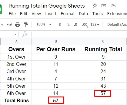
I would like to demonstrate how a running total works or looks before we move on to the formula. Let’s use an example of a cricket match score. However, we all know that during a cricket game, the previous over’s score is added to the current score. So, this could be the most effective way to display a running total to you.
If you’re unfamiliar with cricket scores, then just focus on how the numbers add up sequentially. In this example, column C7 contains the running total from column B2:B7. In other words, C7 equals the sum of all B columns.
Now let’s see how to calculate a running total in Google Sheets using the formulas.
1. Google Sheets’ Cumulative Sum: Normal Running Total Formula
You can use two CUSUM non-array formulas for calculating the running total easily. Let’s see how it works.
Formula 1: Running Total Calculation Using CUSUM Non-Array Formula
There is a formula called the CUSUM available to calculate a running total in your Google Sheets. Let’s see how to-
i. In this process, you can put this formula =sum($B$2:B2) directly in C2 of your Google Sheets. Here, the dollar sign is used to make B2 absolute value.
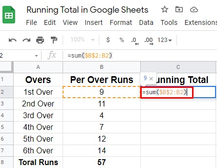
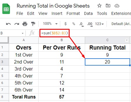
ii. Let’s drag down the formula and see the results accordingly. In cell C3, the formula will look like this =sum($B$2:B3)
Formula 2: Running Total Calculation Using CUSUM Non-Array Formula
This is the easiest way to calculate a running total. You just need to know some easy instructions.
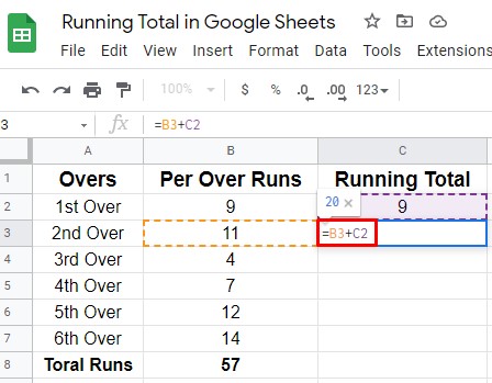
i. Select cell C2 on which you want to have the total and type =B2
ii. Now, in C3, let’s type the formula =B3+C2; by doing so, the summation of the values of both cells reflects. And drat it down eventually. That’s how the process completes.
That’s how you can have your expected running total using these two non-array formulas. Well, let’s start with the array-based formula below.
2. Google Sheets’ (CUSUM) Formulas: Array-based Running Total
You can calculate the running total in Google Sheets using array-based formula as well. Here you’ll get to know 3 three formulas (SUMIF, DSUM, MMULT) through which you make things easier to calculate. Amon three 0f the formula, SUMIF is the most popular one used by many users.
Formula 1: SUMIF – Cumulative Sum Array Formula
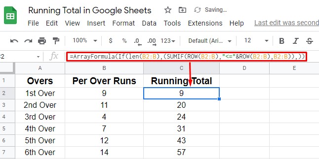
Well, clear the C2 cell at first in your Google Sheets and type or paste the below formula there. And see the magic. Once you put the formula on C2, you’ll get the running total without dragging the formula down to other cells. However, edit or change the cell or column range according to your needs.
=ArrayFormula(If(len(B2:B),(SUMIF(ROW(B2:B),"<="&ROW(B2:B),B2:B)),))
Formula 2: DSUM – Cumulative Sum Array Formula
This is the last cumulative array formula that you can use as well to calculate any kind of running total in your Google Sheets. It’s actually a database function. However, type or paste the below formula in cell C2 as you did before.
And you’ll get your expected results accordingly. However, customize your cell and column range according to your sheets.
=ArrayFormula(DSUM(transpose({B2:B7,if(sequence(6,6)^0+sequence(1,6,row(B2)-1)<=row(B2:B7),transpose(B2:B7))}),sequence(rows(B2:B7),1),{if(,,);if(,,)}))

Formula 3: MMULT – Cumulative Sum Array Formula
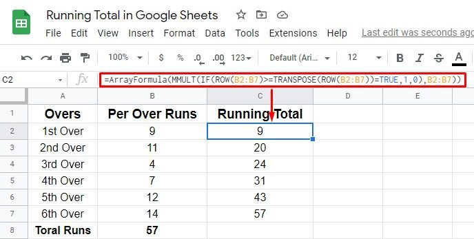
Many users use this MMULT cumulative array formula to calculate the running total in Google Sheets. Here’s the formula below; apply it in cell C2 and easily get the result. No dragging down is also not needed for this formula. However, edit or change the cell or column range according to your sheets.
=ArrayFormula(MMULT(IF(ROW(B2:B7)>=TRANSPOSE(ROW(B2:B7))=TRUE,1,0),B2:B7))
Closing Statement
Well, it’s a wrap. All the functions and formulas have been explained for a running total in Google Sheets. Well, go with any one of them as you wish now. But, I recommend you to go with the SUMIF formula. It’s the most convenient and effective one that is widely used too.
Fro now, I’m taking a leave. Let me know your experience in the comment section below. However, I’ll be back with another Google sheets hack as soon as possible. Furthermore, don’t hesitate to share if you find this needful.
