In Google Sheets, the drop-down list is a unique feature that makes data entry a breeze. You can think of it as a multiple-choice menu. The options will be pre-filled, and you can pick and choose as appropriate. This eliminates the need for repetitive typing of the same thing.
With Google Sheets, you can create a drop-down list for various purposes. As an example, you can update your to-do list as complete, in progress, not started yet. Furthermore, you can create interactive charts and dashboards with drop-down lists.
In the entire article, I will walk you through how to add a drop-down list in different ways, how to paste it from one cell to another, and eventually, how to remove it from your Google Sheets.
How to Add Drop-down List In Google Sheets
You can add a drop-down list in Google sheets in two ways. Using a range of cells and another is a list of items. However both process will work for you, but it has slight differences. I’ll demonstrate that to you, so let’s start.
Method 1: Create a Drop-down using a Range of Cells
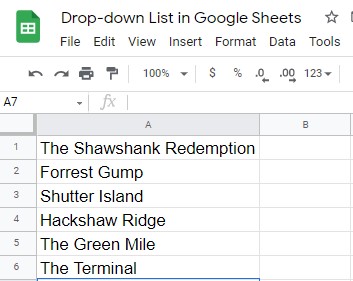
1. To begin with, you need to have a data sheet on which you want to create a drop-down list. For example, see the below attached image. You can see some popular names in it. And it’s in column A1:A6, and I want to create a drop-down list of these movie names in column B using a range of cells. Let’s see how to do that.
2. Well, now select the cell on which you want to have your list and click on the Data menu from the top menu section of your sheets. Find Data validation and click on it.

3. Here is the below page that should be visible to you right now. However, you need to fulfill all the criteria here and finally Save. The criteria should be selected as a List from a range (Sheet1!A1:A6). Now, tik the Show dropdown list in a cell, and Save.
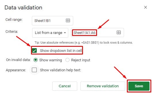
4. What if you want to add more movie names in column A in the future? Is it possible you’ll get those movie names under the drop-down menu then? No, you won’t. Since you have applied dropdown to columns A1-A6, what should you do?
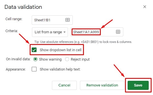
The only thing you need to do is slightly adjust your data validation criteria. Having said that, just make your criteria range Sheet1!A1:A999, and you’re done. Henceforth, your drop-down list will also show the values you might add to column A in the future.
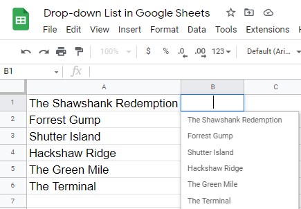
5. What we came up with is below-attached. When you click the first cell in column B (as we selected Sheet1!B1 as the range), the list of values (all the movie names) from column A is displayed.
Method 2: Create Drop-down Manually by Entering the List of Items
If you want to create a drop-down list with static values, you must enter your list of items manually instead of a range of values. Such as Yes/No, Agree/Disagree, and so on. We’ll see how this goes.
1. The first step is to choose the cell you want the dropdown list to appear in. If you want to create on multiple cells, choose accordingly. Now, navigate to Data in the top menu and select Data validation as you did for the previous method.
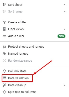
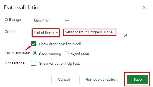
2. You can get the List of items option by selecting the dropdown menu from the first box in the Criteria section. Type your list of values with commas between each value in the next box. However, make sure not to use any space here. Finally, do the rest as before and Save.
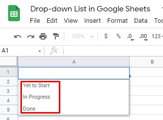
3. Well, here is your drop-down list with values that you typed a few seconds ago. In order to get any value in your cell, click on it, and it’ll appear in your cell.
How To Copy/Paste Drop-down List in Your Google Sheets
So far, we have learned about how to make a dropdown list in your Google Sheets. What if you want to have your drop-down on another column without the Data validation process.
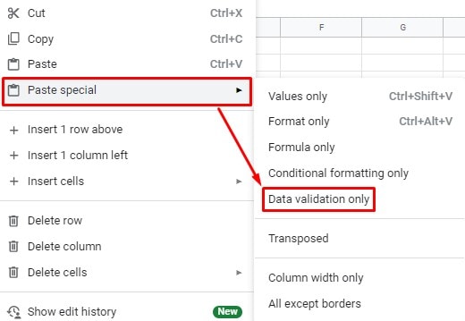
Well, for doing so, you just have to use the Copy/Paste feature. The important thing here is, you need to Paste special and then Data validation only.
At first, copy the drop-down cell, and hover over the cell on which you want to have this list. At this point, select the new cell, click the right button on your mouse. Now navigate the Paste special and Data validation only option from the pop-up options.
Remove Drop-down List from Google Sheets
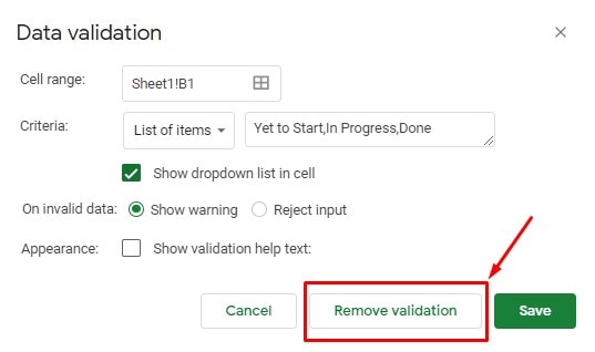
What if you want to delete your drop-down list from your Google Sheets? Simply selecting the cell and clicking on the Delete key from your keyboard won’t do this. To do this, you need to go to the Data validation section again.
You can see the marked section in the below-attached image. So, select the Remove validation and go back to your Google Sheets. And see, there is no drop-down list on your Sheets anymore.
Finally, Insights
To conclude things up, make your data entry work easier than ever. Use Google Sheets drop-down list feature and free yourself from typing the same things repeatedly. Just choose and select with one click on your mouse.
Well, it’s time to take a leave for now. And, I will be back soon with another post which would be needful to you. Let me know your experience on this in the below comment box. And, share with others if you find this needful.
