Usually, you may use the IF function in Google Sheets whenever you need to test any conditions. You can test a condition using the IF function and get the result (based on TRUE or FALSE). What if you have multiple conditions at a time to try? Then, using the IF function will not be a wise decision. Here comes the IFS function in Google Sheets into the play.
Having that said, IFS is the only function to try when you need to test a bunch of conditions within one formula. On the other hand, the IF function can figure out only one condition at a time. Therefore, the IFS function is your only friend in testing multiple conditions in one formula.
In the entire post, I’ll walk you through how you can apply the IFS function in Google Sheets to test multiple conditions in no time. Once you complete the post, you will realize why Google Sheets introduced the IFS function despite already having an IF function.
IFS Function in Google Sheets: Ins and Outs
Well, before showing you the step-by-step process of using the IFS function in Google Sheets, you need to know how this function works, its syntaxes, and how you can use them correctly.
This is how the IFS function looks in your Google Sheets:
=IFS(condition1, value1, [condition2, ...], [value2, ...])
Now, by breaking the syntax down, let me explain each attribute of the function to you so that you can understand it better before using it.
- [=] the equal sign is mandatory to have in any function. With a ‘=’ sign, all the function starts in Google Sheets. Without the equal sign, not any function will work in Google Sheets.
- [IFS] this is the name of the formula. However, we need to add conditions or values in it to work this formula correctly.
- [condition1] this attribute refers to the initial logical test among so many.
- [value1] refers to the expected result of condition1.
- [condition2, value2] these attributes are optional; these refer to the second logical condition and its expected result.
However, following the same procedure, you can keep adding as many conditions and results as you want.
You need to make sure one thing, whatever logic you’re adding should be logically true based on your data.
Points to be Noted while Writing IFS Function
You must remember certain things while writing the IFS function in Google Sheets. Those things are as follows:
- First, you need to know a few signs to make your expressions. For example, you need to use two comparison operators in the function; ‘<‘ less than, ‘>‘ greater than, and also ‘=‘ equal.
- Ensure all the function texts are enclosed using a quote-unquote symbol (“ ”). The numbers can be free; no need to enclose them with the quote-unquote symbol.
- You can’t set a default answer ‘false’ for all the conditions. Whereas you just need to enter ‘true’ at the very last condition.
- Please note that if you don’t use any ‘true’ condition in the function, it results in an ‘#N/A’ error.
Well, there were all the important things about the IFS function.
I’m pretty sure you’ve already become familiar with the function, its attributes, how it works, and what things you need to keep in mind before using it.
However, right now, you might be a bit confused about all these. No worries, now time to show you in practice whatever you’ve learned so far.
Once that is complete, you can easily use the IFS function in Google Sheets.
IFS Functions in a Real-Life Example
Here is an example below where I’ve used the IFS function in Google Sheets. Please give it a look.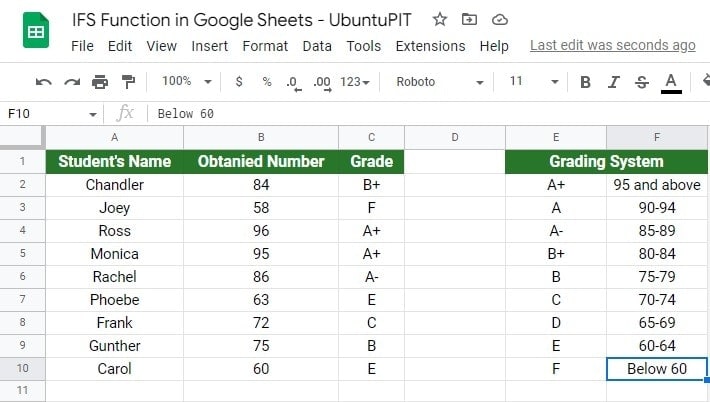 The above sheet contains nine student lists with their obtained mark. And I’ve converted the numeric numbers they scored into a grading system using the IFS function.
As a result, I didn’t have to manually write each student’s grading letters to the individual cell. Instead, one formula did the job for me. Here is the function below that I’ve used here-
=IFS(B2>94,"A+",B2>89,"A",B2>84,"A-",B2>79,"B+",B2>74,"B",B2>69,"C",B2>64,"D",B2>59,"E",B2<60,"F")
Now, allow me to let you know how this function works:
- At first, I selected a cell and clicked on it to make it active after having the data ready to use the IFS function. In my example, that cell was C2.
- After that, I typed with the equal sign to write the IFS function.
- Next, I added the tests or conditions according to the function needs. Based on the Grading System, I figured out the conditions.
- To insert the conditions logically, I used symbols as required. ( > greater than, < less than).
- When I got the cell C2 result, I dragged the result below to cell C10.
And, it’s done! See how easy it was! From now on, you can convert numeric numbers into grades using the IFS function in Google Sheets within a second.
Use IFS Function in Google Sheets (Step-by-Step)
So far, you have learned about the IFS function and saw a real example of using the IFS function in Google Sheets.
However, now I’ll explain to you each step how you can use this IFS function with proper screenshots. Please note that the data set will remain the same for this step-by-step section.
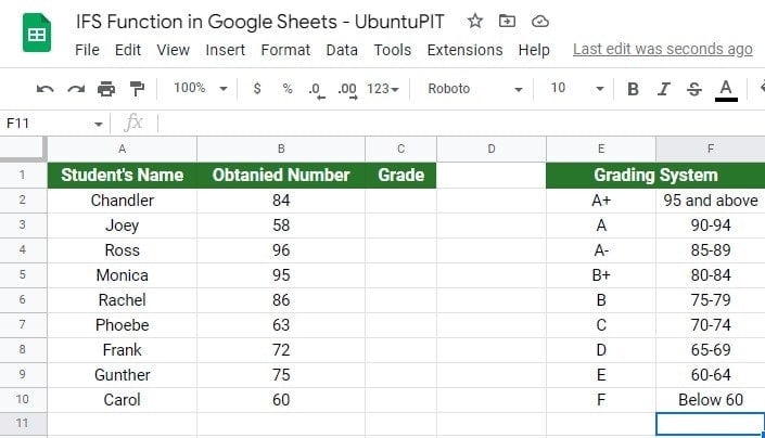
Here is the data set below:
Step 1: Select Any Cell to Write the IFS Function in Google Sheets
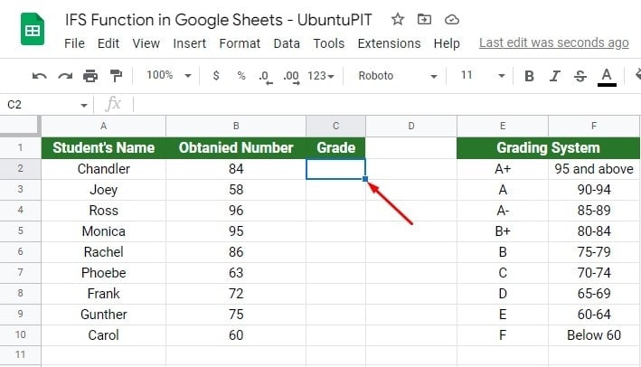
When you have all things ready to use the IFS function in Google Sheets, you need to select a cell where you want to get the result. However, click on the cell to activate it. In my guide, I choose cell C2, where I’ll be writing the formula.
Step 2: Start Writing the IFS Function in Selected Cell
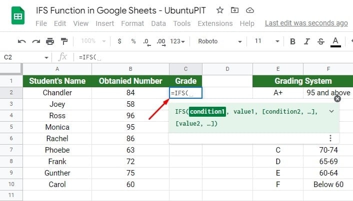
In this step, start writing the formula with the equal sign ‘=‘, and type the function’s name, IFS. When you type the function name, a parenthesis ‘(‘ will open automatically.
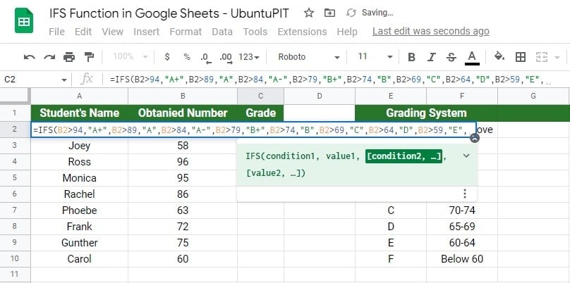
Immediately, you’ll get a pop-up below the cell. Here, you’ll get the function’s syntax, the function summary, and attributes details. These details will guide you in writing the formula correctly.
Step 3: Start with Typing the First Expression
In my guide, I put nine grades under the Grading System. Therefore, the function is supposed to have the exact number of conditions or expressions, too (you might have more or less than nine expressions, it’s totally up to you).
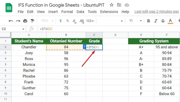
Well, start with typing the first expression. To go with the first expression, you need to call the cell that you want to have there. In my guide, B2 is the first expression cell.
Step 4: Complete the First Expression with Grading System
Once you select your first expression cell, it’s time to add the leftover logical attributes. Having this said, comparison operators will come into play here.
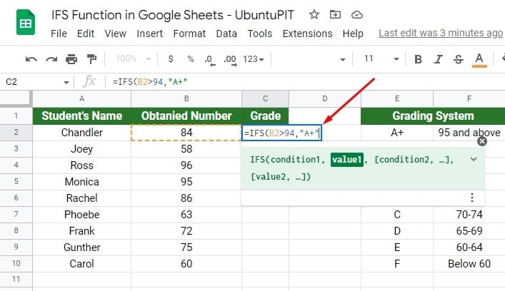
In my guide, the first grading system says, if any student scored 95 or above, they would get an ‘A+’. Therefore, the logic here will be that if the cell B2>94 results in A+.
So, the final expression for cell B2 will be B2>94, “A+” in the formula.
Always make sure you’re using a symbol (” “) in your text string. Otherwise, the IFS function in Google Sheets won’t work at all.
Step 5: Add Remaining Expressions Accordingly
When you complete the first expression, use a comma ‘,’ before adding the second, third, and so on. However, the process will be the same for every expression you want to add to the formula.
In the second expression, write the number 89 (according to the grading system ‘A’) instead of 94. For the second expression, the attribute will be B2>89, “A”.
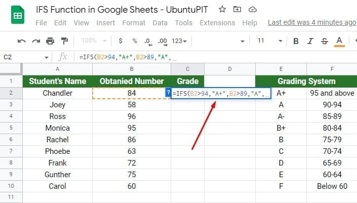
Follow the same procedure for adding the expressions until you reach the nine (the last) expressions. To understand more easily, see the below-attached screenshot.
Step 6: The Last Expression of the IFS Function in Google Sheets
This expression differs from the rest. According to the grading system, the F grade says it will be Below 60. Therefore, you can assume that it’s telling you the number will be 59 or below here.
There is no doubt that a grade of 59 or below is lower than 60. As a result, when you write this expression in the formula, you have to switch the comparison operator from greater than ‘>’ to less than ‘<‘.
Since this is the last step, close the parenthesis ‘)‘ after putting this expression (B2<60, “F”) in the formula.
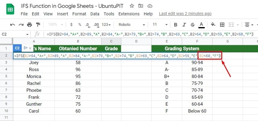
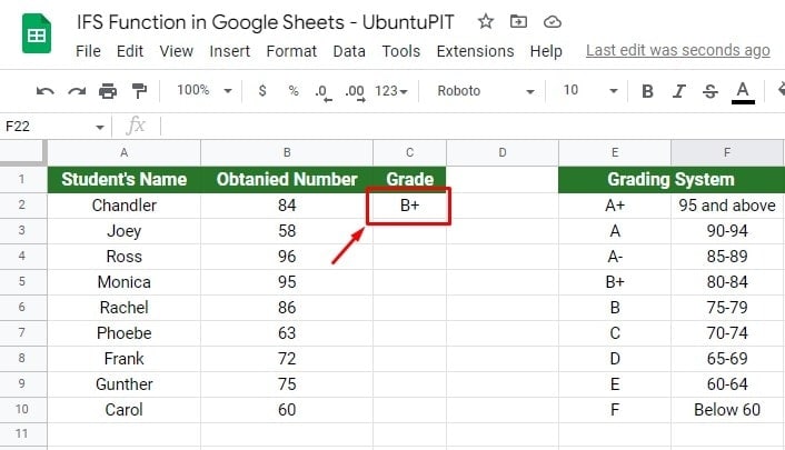
Once you close the parenthesis after putting all the expressions in the formula, hit the Enter button on your keyboard. You’ll get the grade in cell C2 based on your set-up grading system. And see the magic in your cell C2 eventually.
Step 7: It’s Dragging Time
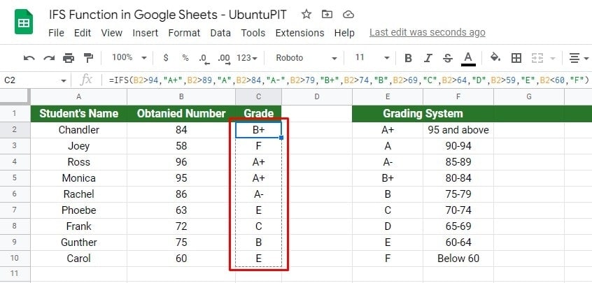
When you get the grading result of B2 in cell C2, drag cell C2 down to cell C10. And, see the magic! By doing so, all cells of column C will be filled up with the grading system you set. Therefore, you don’t need to type formulas in every cell over and over.
Closing Statement, Over to You
There you go! Follow the above steps and use the IFS function in Google Sheets to test multiple conditions within a single formula. However, you can combine other Google Sheets formulas with the IFS to create more effective and potent formulas. Thus, your Google Sheets work will be more accessible than ever before.
Well, usage of the IFS function in Google Sheets ends here. I hope the post helped you. If YES, share this with others and leave your real-time experience in the below comment box. Always be with UbuntuPIT to enhance your Google Workspace knowledge.
