The SORTN function in Google Sheets is ideal when working with massive datasets or catalogs to determine results (for example, the most popular items, top sales, etc.) from those datasets and catalogs. However, having only five or six data items may not require using the SORTN function. But, when you have a large amount of data (e.g., hundreds, thousands), the SORTN function is needed to sort and filter your desired outcome.
Additionally, the SORTN function is a package. Sorting and filtering become so much easier with this function. Moreover, it does not require applying different individual filters. With a function like ARRAY_CONSTRAIN, you can sort dozens of cells in ascending or descending order. But suppose you want the top items, the top sales, the top agents, and more from the catalogs, too? The SORTN function will do it for you.
As of this point, the SORTN function has already been introduced. Well, now let’s look at an example of using the SORTN function in Google Sheets. Before that, we’ll look at how the function works first.
SORTN Function in Google Sheets: An Overview
Every function has its syntax or structure in Google Sheets. And here is the SORTN function syntax below-
=SORTN(range, [n], [display_ties_mode], [sort_column], [is_ascending], …)
Let’s break the function’s syntax down to let you understand each criterion-
- =, This is the first character you need to press on your keyboard to use the SORTN function. As we all know, without the equal sign, no formula is possible in Google Sheets.
- SORTN(), This is the function. Typing this on any cells means you’re ordering your sheets to use this function with all parameters between two brackets.
- range, this is the first parameter. It means the cell range on which you use the SORTN function.
- [n], it indicates a numeric value. The value means the number of results you want from the data.
- [display_ties_mode], this is an optional parameter. You can use several numerical values here according to your needs-
i. 0, you don’t need to write this parameter if you want to go with the default setting. With this mode, you’ll get the top record numbers regardless of duplicates or ties.
ii. 1, you need to use this number when you want to show your top record regardless of duplicates or ties.
iii. 2, it can be used for displaying just one instance of the top records. Let’s assume they have duplicates.
iv. 3, you can use this to return all the top records you already specified along with the duplicates.
- [sort_column], you need to use this parameter when you have the cell ranges with multiple columns. That’s why specifying the column you’ll sort is required.
- [is_ascending], this is an important parameter. You need to type TRUE as the value if you want to sort the ranges in ascending order; on the other hand, type FALSE for the descending order.
An Example of SORTN Function in Google Sheets
An example below is where the SORTN function is used to show you how it works. The function works here to sort and display the top results of the below-mentioned data sheets.
You’ll see that I’ve figured out the top three employee names based on their sales using the SORTN function below.
=SORTN(A2:B11,3,0,2,FALSE)
Now, I’ll tell you the function works here to sort and display the expected results.
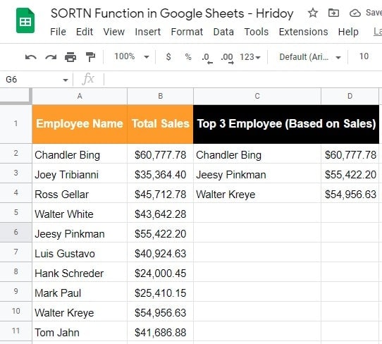
The first parameter includes the employee name and the total sales they have made. And (A2:B11) is the cell range with the employee’s name and sales result.
Moreover, the numerical number 3 after the range is used here to let the function know that I wished to get the top three employee results with the highest-selling records.
After that, I used numerical number 2 as the [sort_column] parameter to let the SORTN function know that I’m setting column B as the criteria from where I like to get the top three employees with the highest sales.
Lastly, I’ve typed in the function [is_ascending] as a parameter, which holds FALSE. However, I’ve used this value as FALSE so that I could get the sorted results in descending order.
So here is a short explanation below of this example:
The SORTN function works and provides the result based on the given parameters. And, then according set values, the function sort and display the top the employee results with the highest sales record. It’s super easy, right?
Well, I think you understood how the SORTN function in Google Sheets works. However, let me make things more transparent by showing you the step-by-step process in the following section.
How to Use the SORTN Function in Google Sheets
Here is the step-by-step process below to show you how the SORT function in Google Sheets works.
Step 1: Select the Cell and Start Applying the SORTN Function
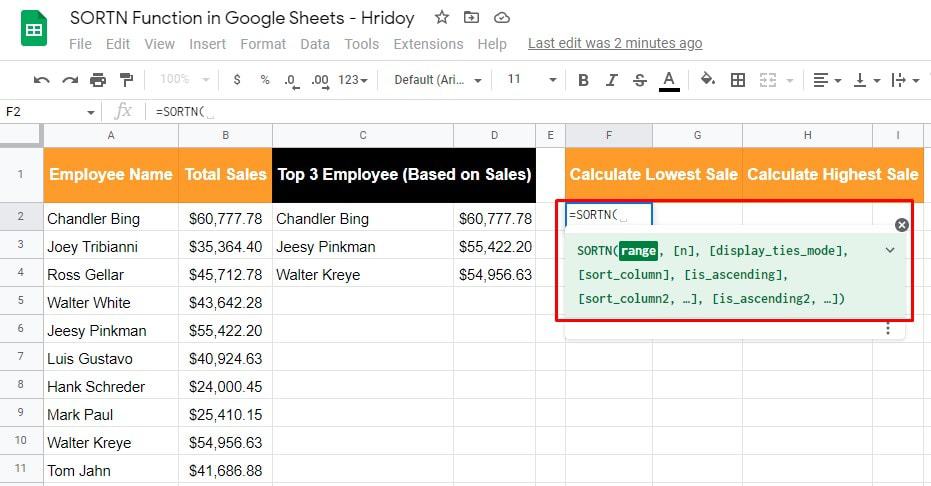
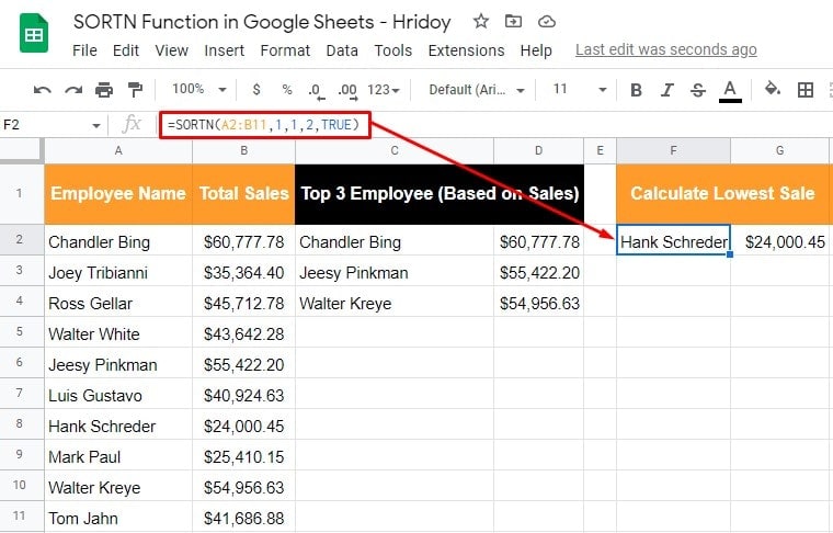
To show you how the function works, I added two new columns with the heading Lowest Sale and Highest Sale. At first, click the cell where you want to have the result.
However, let’s find out the lowest sale first. And to start this, I choose cell F2.
When you click on cell, the cell will be ready to take the function. Start with the ‘=’ equal sign and the name of the function, SORTN.
You’ll notice that the moment you type the function name, an auto-suggest box will appear with all the criteria that require to work the function.
Step 2: Start Inserting the Parameters of the Function
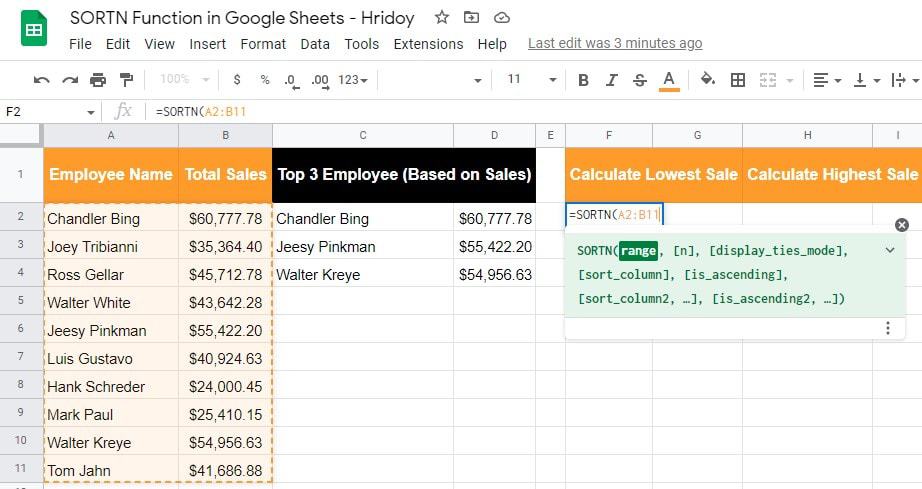
It’s time to put the required parameters of the function. To begin, set the cell range with the data from where the function sort.
So, I have added all the data, including all the employee names and sales records. So, the cell range for this example sheet is A2:B11.
N.B: Please note, in Google Sheets, you can choose the cell range in two ways. Either you type it manually or drag over the cells you need.
So, you can choose whichever way you want. Plus, you’ll notice a highlighted color on your Google Sheets’ selected cells whenever you choose the cell range.
Step 3: The Number of Records You Wish to Get Return
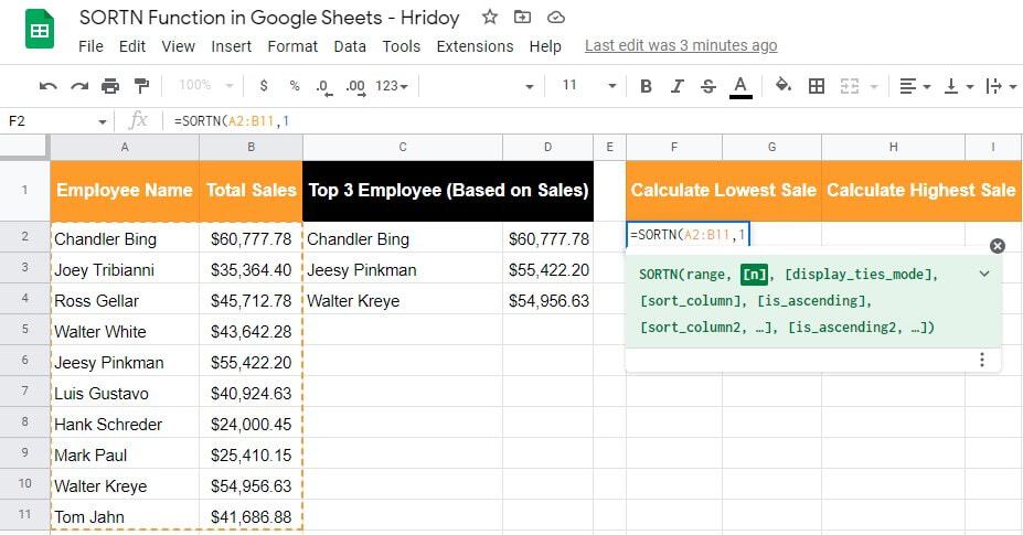
This parameter defines the number of records one would like to get back as a result. Since I’m going to figure out the lowest sale, the following parameter will be 1 for [n] in the syntax.
Step 4: Inserting Display Ties Mode Parameter
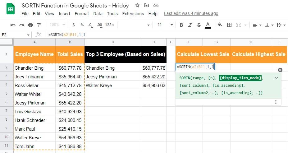
A tie in the total sales results among all the employees could be possible. Therefore, [display_ties_mode] parameter needs to set as 1.
As I said above, the function having 1 for this parameter will also show the result with all ties.
Step 5: Select the Column from Where to Start Sorting
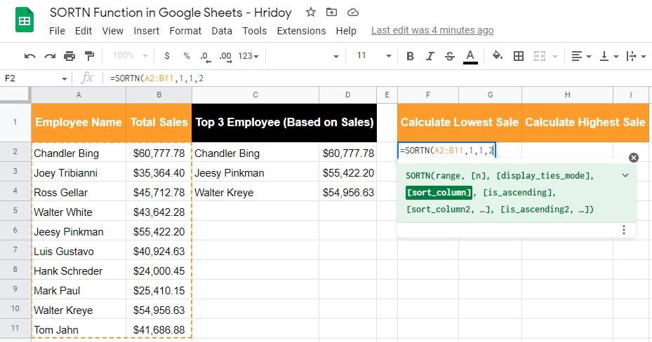
There is doubt that you must select the column from where the sorting process starts. As per the demo data, column B has the sales record data and is in the second column of the range. Therefore, as [sort_column], I enter 2 in the function.
Step 6: Set the Sorting Order (Ascending or Descending)
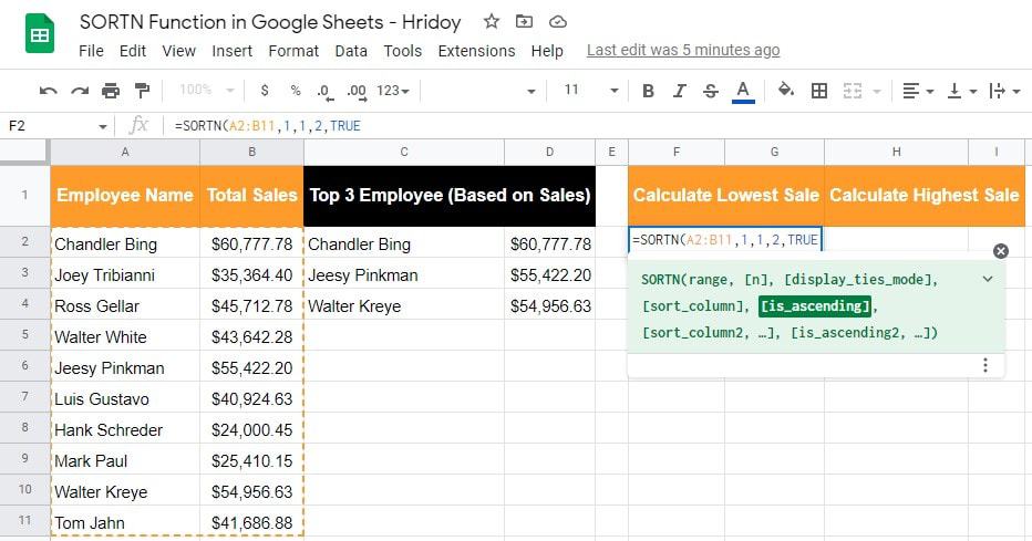
The last parameter of my demo sheet is [is_ascending], which defines the data sorting process. As I mentioned, I’m figuring out the lowest sale. Therefore, the sorting order should be ascending (lowest to highest).
However, this parameter decides whether the sorting process will be ascending or not. And here could be two possibilities- TRUE or FALSE. And to verify that the soring process will be ascending, you must enter TRUE here.
Step 7: Close the SORTN Function and Get the Lowest Sale Result
The last step will be closing the function. And to do this, you must type the right side closing parenthesis ‘)’ in the function. Since you input all the requirements, now is time to click on the Enter button.
As a result, you will have an output like the below one. Finally, you’ll get the lowest result that you are looking for in your Google Sheets.
Step 8: Let’s Get the Highest Sale Value Using SORTN Function
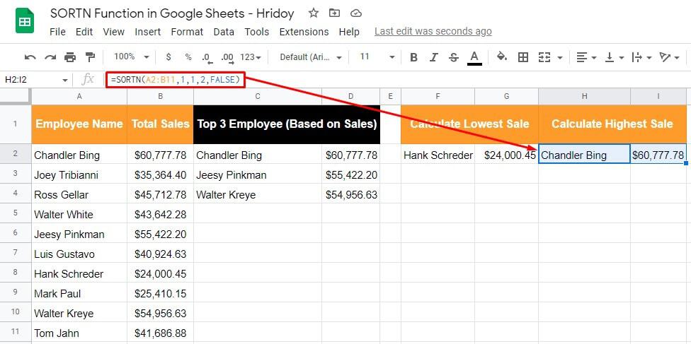
Finding the lowest result was easy, right? I think it was. However, you could get the highest result using a similar manner. This time, I took the H2 cell to display the highest result.
And to do it, you must apply the same procedure discussed above except for one slightest change. That is, you have to set [is_ascending] to FALSE.
However, you’ll get a result like the one below that contains the highest sales record only if you correctly use the SORTN function in Google Sheets.
Closing Statement
Well, that’s how everything completes here. From now onwards, you can easily use the SORTN function in Google Sheets. Once you master this function, filtering and sorting from massive data to get the expected result will be super easy.
Therefore, if you want to filter and sort any top result from a massive datasheet or catalogs in ascending or descending order, going with the SORTN function could be the only choice.
Moreover, you can use this SORTN function along with many other Google Sheets functions to make your work complete. I hope this will help you to streamline your work.
However, let me know your feedback on this and share it if you find it worth sharing. Well, taking leave now. Be a regular reader of UbutuPIT, and I’ll be back soon with another one.
