Google Sheets offers tons of functions and formulas. Among them, the ARRAY FORMULA function in Google Sheets is the most effective and versatile one, without any doubt. Could you please let me know one thing, honestly? Did you ever create and apply any formula to a particular cell and then copy or drag that to the corresponding cell for the result? I bet you did.
However, the ARRAY FORMULA will make your work easier. You don’t need to copy or drag your formula to the adjacent cell anymore. Because, using a single ARRAY FORMULA function in Google Sheets, you can get a range of cells (including rows and columns) result in no time. Therefore, you can say goodbye to the copying and dragging method.
Having all this said, I’ll be with you for the entire article to show you the ARRAY FORMULA function and how the ARRAY FORMULA function in Google Sheets works.
The ARRAY FORMULA Function in Google Sheets
ARRAY FORMULA function calculates multiple rows/columns with a cell range at a time. Besides, you can automate the function too.
For example, the function will update automatically when you add new values to any column or row. And to do this, you just need to set your ARRAY FORMULA function accordingly.
Moreover, the ARRAY FORMULA function also works with non-array functions (e.g., IF, SUMIF, SUM, FILTER, or VLOOKUP). Thus, you can collaborate easily to sort out any complex calculations quickly.
An Example of ARRAY FORMULA Function in Google Sheets
For better understanding, let me show you an example where I used the ARRAY FORMULA function for different purposes.
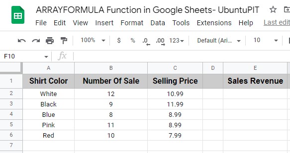
The below example data contains different Shirt items with their sale price and number count of the sales.
And a Sales Revenue column is there, where I want to calculate sales revenue for each item and the total sales revenue of all the shirt items. How do you do these?
Usually, in a scenario like this, you may create a formula to get the sales revenue result by multiplying columns B and C, then paste that down to the row number you want to, and finally sum all the rows together.
However, you can use the ARRAY FORMULA function instead of using this conventional method as I did.
Get Sales Revenue of Each Row
As you can see, five rows are in the data sheet with values. Let’s assume you want to get each row’s sales revenue by applying one single formula.
Yes, I’m talking about the ARRAY FORMULA function in Google Sheets.
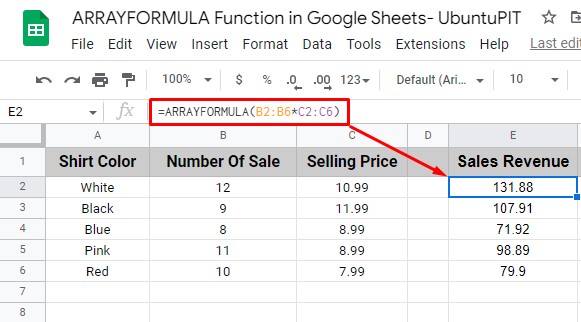
Now, click on cell E2 (1st row of Sales Revenue column) and type this =ARRAYFORMULA (B2:B6*C2:C6). Once you type the entire data range in the function attribute, hit Enter button.
See the magic! There you have each item’s sales revenue by just using one formula.
Get the Entire Sum of Sales Revenue
In this section, I’ll show you how you can get the total sum of the sales revenue using just one formula, the ARRAY FORMULA function.
However, since you’ll be calculating the total sales revenue, you need to use the SUM function with the ARRAY FORMULA function.
Having this said, below is the formula (based on my data sheets) you need to type once you select the cell where you want to get the entire sum of the sales revenue.
=ARRAYFORMULA(SUM(B2:B6*C2:C6))
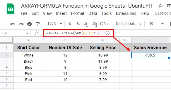
This is how you can get individual rows’ sales revenue and then sum them up for total sales revenue by using just one amazing ARRAY FORMULA function in Google Sheets.
Well, the following section will be the step-by-step procedure on how you can use the ARRAY FORMULA function in Google Sheets.
How to Use ARRAY FORMULA in Google Sheets
Before going to show you the step-by-step process of how you can use the ARRAY FORMULA function in Google Sheets, let me inform you of the syntax of this function.
The Syntax of the ARRAY FORMULA
Here’s the ARRAY FORMULA syntax
=ARRAYFORMULA (array_formula)
array_formula, which refers to the same size cell ranges (one or more) mathematical expressions.
However, the ARRAY FORMULA in Google Sheets works with any mathematical expression. You just need to ensure one thing: the cell ranges need to be the same size all the time. That’s it!
Well, let me clear this more. I used the ARRAY FORMULA function above in my demo data sheet to get the entire sum.
=ARRAYFORMULA(SUM(B2:B6*C2:C6))
What if I type B4 instead of B6 in this formula? Yes, the cell range will not be the same size then. If I do this, I’ll get an error in the ARRAY FORMULA.
Therefore, keeping the cell ranges of the same size is a must while using the ARRAY FORMULA function in Google Sheets.
Calculate Entire Column Result Using the ARRAY FORMULA
There is only one formula available in Google Sheets to apply to an entire column, ARRAY FORMULA.
Therefore, when you enter any new column value, later on, the ARRAY FORMULA function will automatically work with those values to provide the expected result.
Let’s have a look at the step-by-step process below:
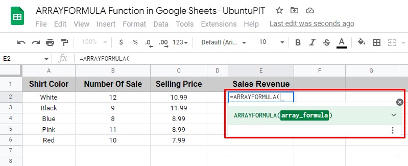
1. First, pick a cell on which you want to apply the formula. After that, click on the equal sign (=) to start the formula. Now type ‘ARRAYFORMULA’ in the cell and click on Tab.
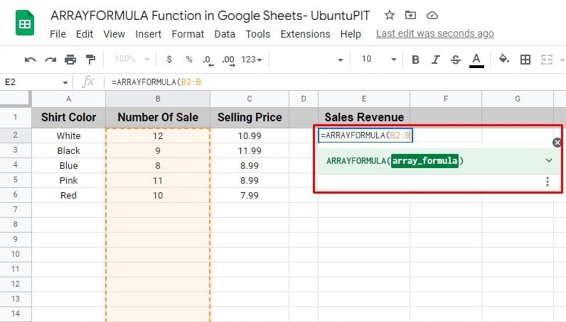
2. Select the first column attribute (B2) you want to add to the formula. However, if you would like to apply the formula to the entire column, type the column name (B) after “:” without specifying any particular cell number.
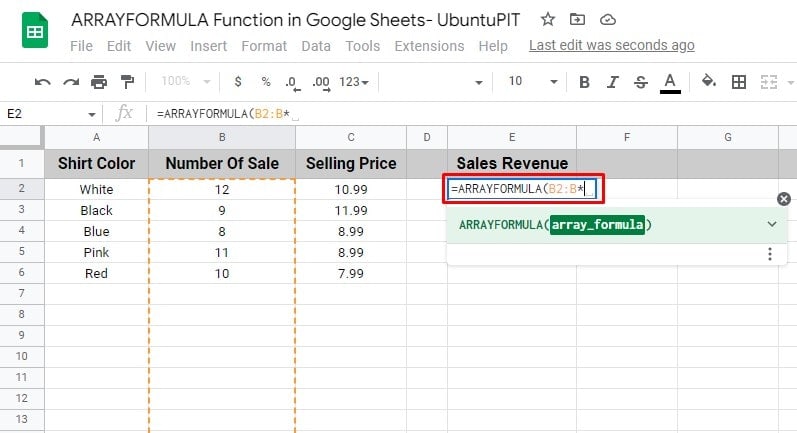
3. Now, before picking another column, now put the mathematical operator or function in your formula. In my example, I’m multiplying two columns. Therefore, I used “*” after selecting the first column range.
4. Insert your second column cell range in the formula. If you want to select the entire column, do the same as you did for the first column.
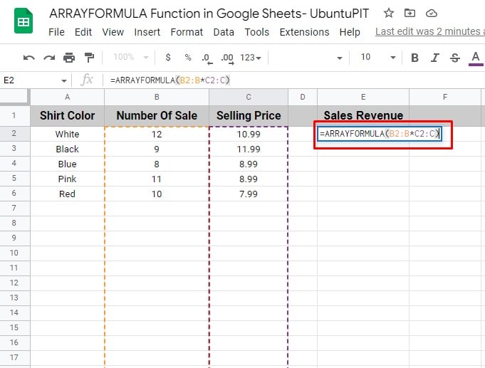
5. Once you put the attributes in your formula, close the formula and hit the Enter button. Thus, the formula will calculate and provide the result based on the expressions you set.
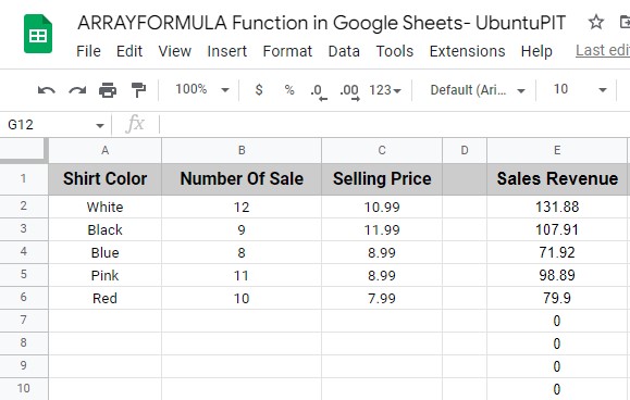
N.B: When you need to calculate any entire column using any formula, the ARRAY FORMULA function is the quickest one.
But a question may arise, why is the 0 there in the entire column? It’s because those rows don’t contain any values.
However, when you put any values, the formula will automatically calculate. Or else, if you don’t need this, select your cell ranges up to where you have data.
Wrap the ARRAY FORMULA Automatically Using Keyboard Shortcut
You can use a keyboard shortcut to wrap the ARRAY FORMULA function in Google Sheets automatically. Here is the keyboard shortcut below:
CTRL+SHIFT+ENTER
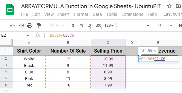
In the below example, I’ve multiplied the column range of B and C. I started the formula with an equal sign and put the attributes accordingly.
After that, press the shortcut key mentioned above. When I pressed the shortcut key, the entire formula automatically wrapped up in the ARRAY FORMULA function.
Usage of ARRAY FORMULA in Google Sheets with IF
As I said earlier, you can use the ARRAY FORMULA function in Google Sheets with other non-array formulas. By far, this is the best feature of the ARRAY FORMULA function.
Having said this, IF is the non-array function commonly used with the ARRAY FORMULA function now and then for different purposes.
Therefore, I’ll show you an example here of how you can combine the If and ARRAY FORMULA functions together.
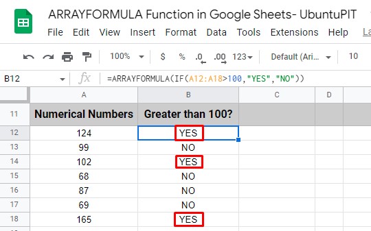
As you can see, the IF function is being used with the ARRAY FORMULA function in the below example datasheet.
Let’s assume you want to get the results that are more than 100 in column A, using the IF and ARRAY FORMULA function together. To do so, you need to follow the below simple steps.
1. You need to have your IF statement in column A first.
2. Now, select a cell where you want to get the result. In my example, I picked cell B2. Write your IF function there, and wrap the entire IF function part inside the ARRAY FORMULA.
3. When you complete the function, hit the Enter button on your keyboard. There you have the result based on YES and NO. If greater than 100, “YES”, and if less than 100, “NO” results will appear in column B, as you set your IF function.
Closing Statement
That is how everything completes. It’s pretty clear that you can make your work easier and faster by using the ARRAY FORMULA function in Google Sheets. Due to its versatile functionalities, you can also use this with non-array functions.
Therefore, drop your conventional way of copying and dragging the formula to the entire range of cells and use the ARRAY FORMULA function instead.
That’s it for now. I’ll be back soon with another one. Please let me know your valuable feedback in the comment section mentioning your experience with this post.
Besides, sharing it with others will be much appreciated. However, share this post only if you find this helpful for you. Be with UbuntuPIT, be informative because this matters the most nowadays.
